Code
df <- read.csv('NYPD_Complaint_Data_Current__Year_To_Date_.csv')
df[df == "(null)"] <- NA
#dfThis dataset includes all valid felony, misdemeanor, and violation crimes reported to the New York City Police Department (NYPD) for all complete quarters so far this year (2023). This data is manually extracted and reviewed by the Office of Management Analysis and Planning.
Each record represents a criminal complaint in NYC and includes information about the type of crime, the location and time of enforcement. In addition, information related to victim and suspect demographics is also included.
The data is provided by NYPD and is updated quarterly. It was made public in November 2018.
We can download the data from the NYPD and import into R as a csv file. Go to “export”, then download as CSV. It can be downloaded from: https://data.cityofnewyork.us/Public-Safety/NYPD-Complaint-Data-Current-Year-To-Date-/5uac-w243/data
There are 415310 rows and 36 columns. Important columns include:
Location:
Precinct where incident occurred
Borough where incident occurred
Patrol borough in which incident occurred
Premise (grocery store, residence, street, etc)
Location at premise (inside premises, front of, rear of, etc)
Transit station name
Parks: NYC park, greenspace, playground, if applicable
NYCHA housing development level
Latitude/Longitude
Crime details:
Date of incident
Time of incident
Level of offense (felony, misdemeanor, violation)
Crime success (indicates if crime was successful or failed)
Jurisdiction responsible for incident (ex: police, transit police, long island rail road, etc)
Individuals’ info:
Suspect’s Age group
Suspect’s race
Suspect’s sex
Victim’s age group
Victim’s race
Victim’s sex
There are also end date and end time columns, which are populated if initial date and time are not known. We will have to handle the rows where the exact timing of the crime is unknown.
We have details on the location, date, time, type of crime, premise, jurisdiction responsible, and crime success. We can look at the frequency of different crime levels across locations, premises, dates, and times. The location information (including latitude, longitude, and precinct) would allow us to plot a heatmap on top of the NYC map (which we can access from publicly available datasets in the form of shapely files) and visualize which neighborhoods are most prone to crime and which types of crimes are more prone in certain areas. The temporal information (including the date and times) could allow us to plot a timeseries graph to uncover insights on seasonal changes on different types of crime. This will shed insight on what parts of the year or day of the week are prone to certain types of crimes. Not only that, we can also compare different crime levels across victim age, race, and sex to observe if there is a correlation between age, race and sex to chance of being victimized by crime. We can also plot the frequency of successful crimes to failed ones across jurisdictions to analyze how often crimes are successful, and which jurisdiction fails or succeeds to stop them. This would also allow us to see what type of crimes are least likely to be committed successfully and at which times of the year and what locations within NYC.
Here we will plot only the columns that have null values. The other columns don’t have any null values:
df <- read.csv('NYPD_Complaint_Data_Current__Year_To_Date_.csv')
df[df == "(null)"] <- NA
#dfis_na <- is.na(df)
missing_counts_sum <- colSums(is_na)
missing_counts_percent <- colMeans(is_na)
plot_data_sum <- data.frame(
column = names(missing_counts_sum),
missing_count = missing_counts_sum
)
plot_data_sum$column <- factor(plot_data_sum$column, levels = plot_data_sum$column[order(plot_data_sum$missing_count)])
plot_data_percent <- data.frame(
column = names(missing_counts_percent),
missing_count = missing_counts_percent
)
plot_data_percent$column <- factor(plot_data_percent$column, levels = plot_data_percent$column[order(plot_data_percent$missing_count)])#print(nrow(df))library(ggplot2)
ggplot(plot_data_sum[plot_data_sum$missing_count > 0, ], aes(x = column, y = missing_count)) +
geom_bar(stat = "identity", color = "black") +
labs(title = "Number of missing values", x = "Column Names", y = "Counts") +
theme_minimal() +
coord_flip()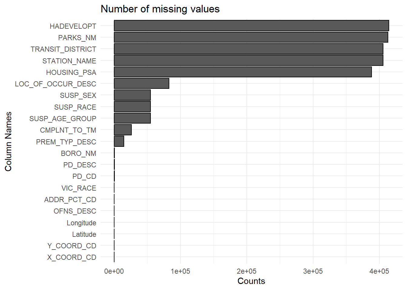
ggplot(plot_data_percent[plot_data_percent$missing_count > 0, ], aes(x = column, y = missing_count)) +
  geom_bar(stat = "identity", color = "black") +
  labs(title = "Percent of missing values", x = "Column Names", y = "Percentage") +
  theme_minimal() +
  coord_flip()
There are some columns with almost all values missing: Hadevelopt, Parks_nm, Transit_district, Station_name, Housing_psa
Hadevelopt is the name of the housing development occurrence, and housing_psa is the development level code. This just means that almost all the crimes don’t happen around housing development. This makes sense since housing development in NYC is very scarce (one of the reasons housing is very expensive in the city).
Parks_nm indicates if the crime happened in a park or playground, so null values indicate most crimes did not happen in these areas. The same reasoning can be applied for null values for Station_name (indicating a subway station) and transit_district (district code for subway station).
For these columns, missing values just indicates the crime did not occur at that particular location. Since almost all the values are missing, we can drop these columns. We have another column that describes the location of the crime, so we aren’t losing any valuable information by dropping these.
filtered_rows <- df[is.na(df$LOC_OF_OCCUR_DESC), ]
category_counts <- table(filtered_rows$PREM_TYP_DESC)

barplot(category_counts[category_counts>6000], main='Null premise location occurrences',
        xlab = 'category',
        ylab= 'count')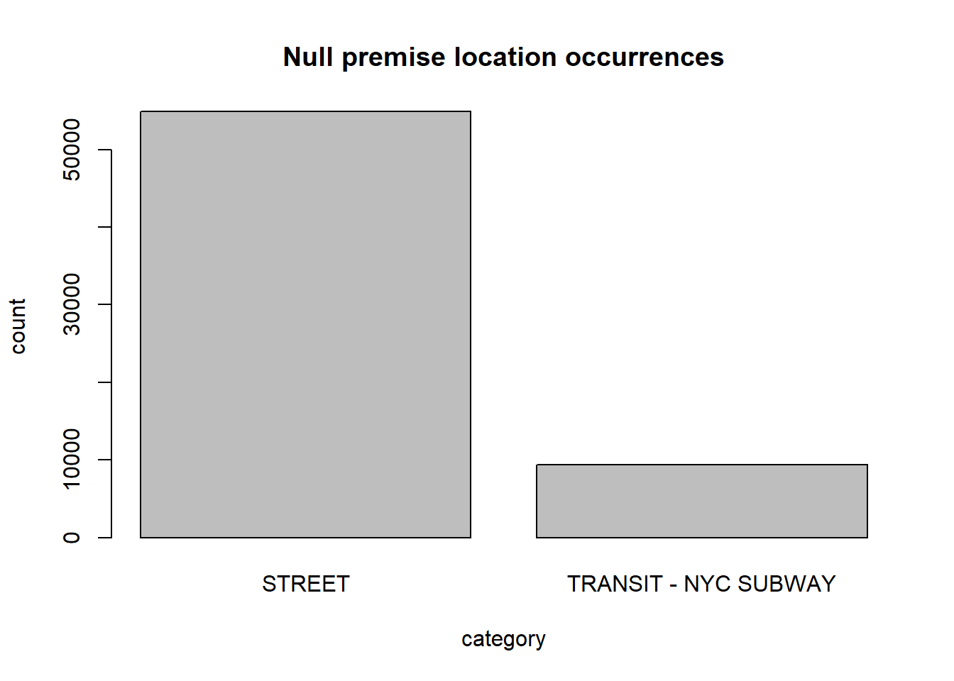
Loc_of_occur_desc indicates if a crime occurred inside, in front of, or behind a premise. We noticed the null values happen when the premise is either the street or an NYC subway, so the exact location around the premises doesn’t make sense. We can probably drop this column since the information is not that useful.
Let’s use another plot to examine the smaller missing values.
ggplot(plot_data_sum[plot_data_sum$missing_count > 0 & plot_data_sum$missing_count < 60000, ], aes(x = column, y = missing_count)) +
  geom_bar(stat = "identity", color = "black") +
  labs(title = "Number of missing values (below 60000)", x = "Column Names", y = "Counts") +
  theme_minimal() +
  coord_flip()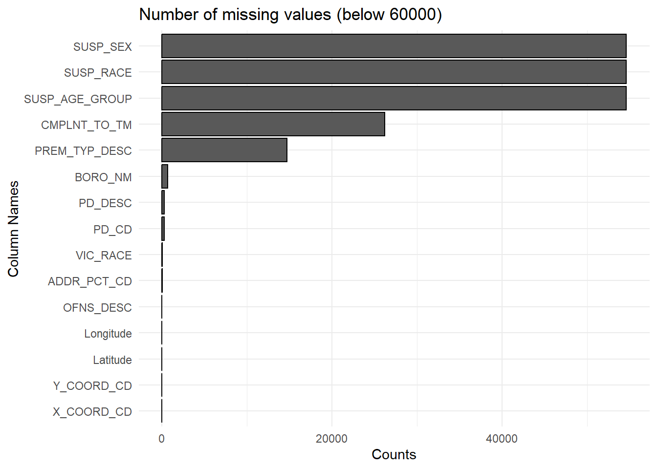
The count of missing values for suspect sex, race, and age group are the same. This indicates that the suspect got away with the crime. We should examine this data later to see if there is a trend for suspects who escaped, so let’s keep these missing values.
ggplot(plot_data_sum[plot_data_sum$missing_count > 0 & plot_data_sum$missing_count < 700, ], aes(x = column, y = missing_count)) +
  geom_bar(stat = "identity", color = "black") +
  labs(title = "Number of missing values (below 700)", x = "Column Names", y = "Counts") +
  theme_minimal() +
  coord_flip()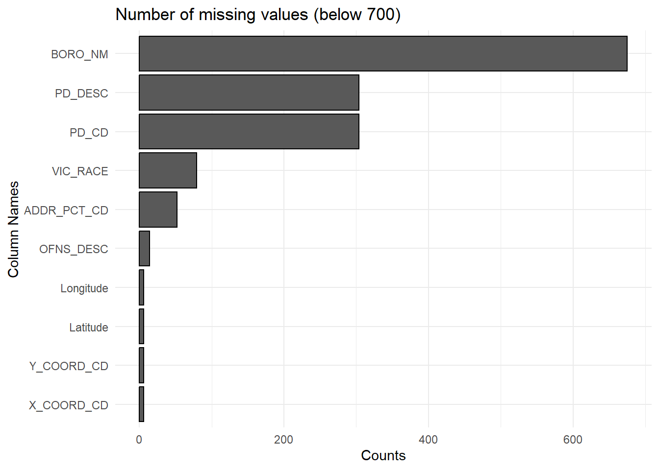
The rest of these missing values are very minimal compared to amount of data we have. We can just drop these rows since missing values make up only about 1% for these features.
df$Date <- as.Date(df$CMPLNT_FR_DT, format = "%m/%d/%Y")

df <- df[order(df$Date), ]

ggplot(df, aes(x = Date)) +
  geom_histogram(binwidth = 7, fill = "skyblue", color = "black", alpha = 0.7) +
  geom_vline(xintercept = as.Date("2023-01-01"), linetype = "dashed", color = "red", linewidth = 1) +
  labs(title = "Date Counts Histogram", x = "Date", y = "Count") +
  xlim(as.Date('2022-01-01'), max(df$Date)) +
  theme_minimal()
Warning: Removed 2197 rows containing non-finite values (`stat_bin()`).Warning: Removed 2 rows containing missing values (`geom_bar()`).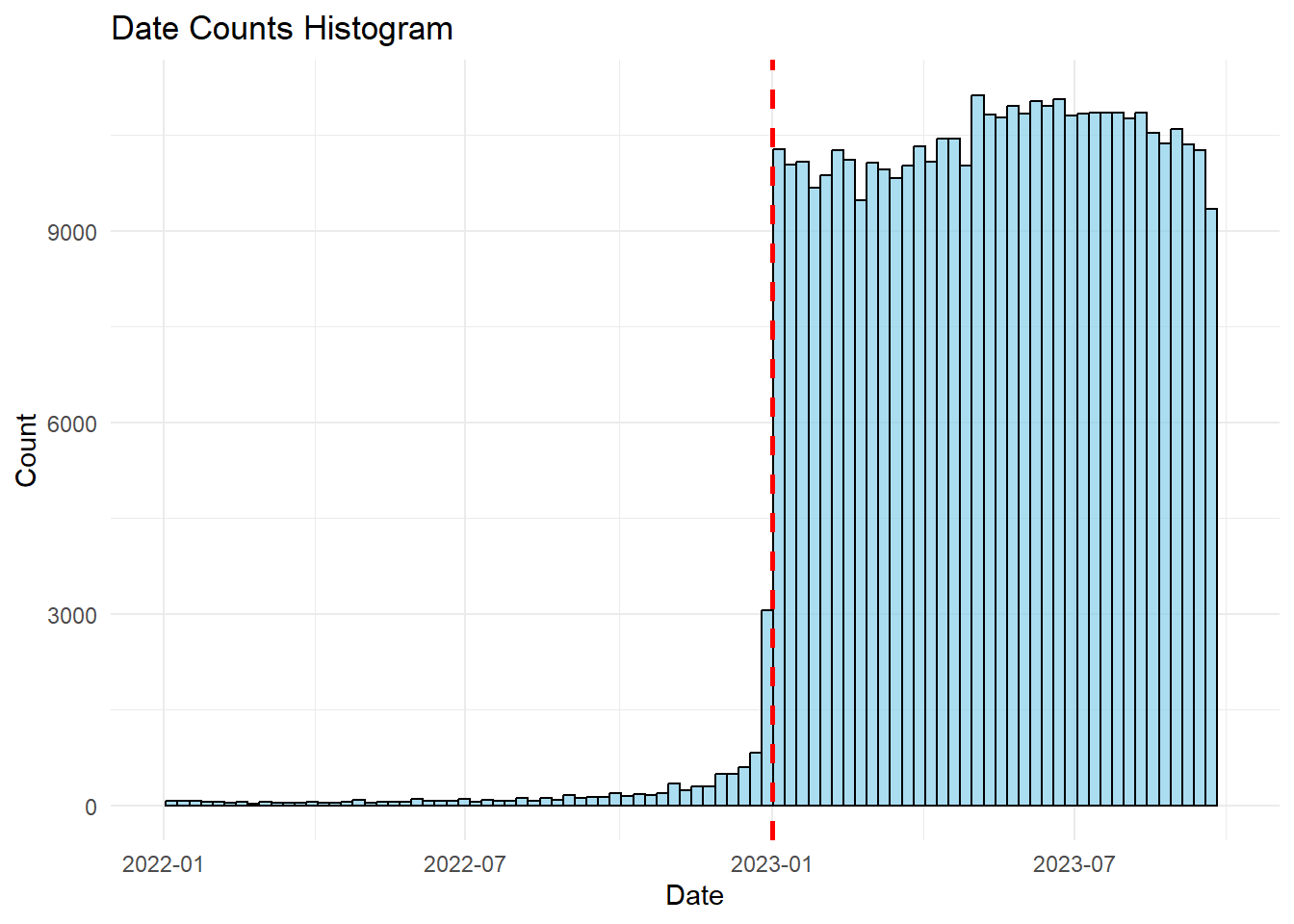
A significant proportion of the recorded crimes happened in the year 2023. The data from 2022 is underrepresented, therefore we’ll only use data from 2023.